3. Basic fractal information 

Table of contents


 3a. 

What is a fractal? What are some examples of fractals? 


 3b. 

Where can I find more information about fractals on the web? 


 3c. 

Are there natural fractal structures? 


 3d. 

What are the main different types of fractal images? 


 3e. 

What are recursion and iteration? 


 3f. 

What are iterated complex polynomials? 


 3g. 

What is an iterated function system (IFS)? 


 3h. 

What is a strange attractor? 


 3i.  

What are flame fractals? 


 3j. 

What are L-systems? 


 3k. 

What are fractal terrains? 


 3l.  

What is fractal music? 


 3a

What is a fractal? What are some examples of fractals? 


   A fractal is a rough or fragmented geometric shape that can be subdivided in parts, each of which is (at least approximately) a reduced-size copy of the whole. Fractals are generally self-similar and independent of scale.
   There are many mathematical structures that are fractals; e.g. Sierpinski triangle, Koch snowflake, Peano curve, Mandelbrot set, and Lorenz attractor.
   Benoît B. Mandelbrot gives a mathematical definition of fractal as a set for which the Hausdorff Besicovich dimension strictly exceeds the topological dimension (this will be explained later). However, he is not satisfied with this definition as it excludes some sets that could be considered fractals.
   According to Mandelbrot, who invented the term:

I coined fractal from the Latin adjective fractus. The corresponding Latin verb frangere means “to break”: to create irregular fragments. It is therefore sensible - and how appropriate for our needs! - that, in addition to “fragmented” (as in fraction or refraction), fractus should also mean “irregular,” both meanings being preserved in fragment. (The Fractal Geometry of Nature, page 4)


 3b

Where can I find more information about fractals on the web? 


   There are many good fractal articles and tutorials available at different sites. Several useful links are given in each of the corresponding sections of this FAQ, but you can also use a search engine, with appropriate keywords, to spark off your interest or curiosity.
   If you think links to new web pages deserve to be added to this FAQ you are encouraged to submit them, but the editors may or may not include them, depending their interest and the redundancy of the material with respect to already existing links. If better, a new link may replace a previous one.
   This FAQ does not intent to offer an exhaustive list of all the links related to the topics evoked. Several sites have such lists and are cited here:


 3c

Are there natural fractal structures? 


   Yes, fractals describe many real-world objects, such as clouds, mountains, coastlines, roots, branches of trees, blood vessels, and lungs of animals; perhaps the structure of the universe itself... (all those structures do not fit into simple geometric shapes). They can also describe quite well natural phenomena such as percolation of liquids in porous materials (like soils), distribution in the time of  river floods, Brownian motion...
   It is worth noting that the title of the underlying French book of Dr. Mandelbrot was “Les objets fractals” and its English equivalent was “The fractal geometry of nature”.


 3d

What are the main different types of fractal images? 


   Fractals can be subdivided into several groups. The following list does not pretend to be exhaustive.

  • Fractals derived from standard geometry by using iterative transformations on an initial common figure like a straight line (the Cantor dust or the von Koch curve), a triangle (the Sierpinsky triangle), or a cube (the Menger sponge). The first fractal figures invented near the end of the 19th and early 20th centuries belong to this group.
  • IFS (iterate function systems).
  • Strange attractors.
  • Flame fractals.
  • L-system fractals.
  • Fractals created by the iteration of complex polynomials:  perhaps the most famous fractals.
  • Quaternionic and (recently) hypernionic fractals.
  • Fractal terrains generated by random fractal processes.


 3e

What are recursion and iteration? 


   An iteration is a mathematical (or geometrical) operation that is repeated a certain number of times to reach (or approximate) the final result. The division of 10 by 3 gives a result of 3 and a remainder of 1. The division of 1 by 3 gives a result of 0.3 and a remainder of 0.1. The division of 0.1 by 3 gives a result of 0.03 and a remainder of 0.01. Therefore 3+0.3+0.03...=3.33... is the approximate value of 10/3 and you see that the division algorithm is iterative.
   Now, suppose an operation giving certain result and an iteration which applies the same operation to the result itself: this iterating process is recursive. This can be illustrated in a simple way by the process used to obtain the Cantor dust:
   Start with a straight segment, the length of which is L. Remove the central 1/3 of this segment. That leaves you  2 segments of length L/3. Remove the central 1/3 of each segment, and you get 4 segments of length L/9. Repeating this recursive process endlessly leads to the Cantor dust, perhaps the most simple fractal.

from Third Apex to Fractovia.(http://www.fractovia.org/what/what_ing1.html)

   The algorithm can be written as follows:

let a segment L;
Beginning of the procedure "Cantor"
 (to apply to any segment);
    erase the central 1/3 of the segment;
    do again the procedure "Cantor" on the resulting
     segments (this is the recursion);
End of the procedure;

   The Cantor procedure contains a call to itself. Therefore, it repeats itself endlessly on every segment obtained by the previous call. If you try to execute this procedure with a computer, it will never stop! That’s why it is necessary to add a stopping condition after a given number of iterations.

let a segment L;
let N be equal to 0;
Beginning of the procedure "Cantor" (to apply to any segment);
   let N be N+1 (N is a counter);
   if N=10 (or any other number) then exit the procedure 
    (stopping condition);
   erase the central 1/3 of the segment;
   do again the procedure "Cantor" on the resulting
    segments (this is the recursion);
End of the procedure;

   Now, the procedure will stop after 10 iterations.
   What we have written is known as a pseudo-code (too verbose indeed, but this is necessary for readers who are not familiar with computer programming). It can easily be translated to any programming language to be run with a computer.
   All fractals are obtained by recursive procedures. For example a little change in the previous procedure will give the von Koch curve:

let a segment L;
let N be equal to 0;
Beginning of the procedure "Koch";
   let N be N+1;
   if N=10 then exit the procedure;
       erase the central 1/3 of the segment;
       replace it with 2 segments of length 1/3;
       do again the procedure "Koch"
        on the resulting segments;
End of the procedure;


 3f

What are iterated complex polynomials?


   Complex polynomials are used to draw the well known images of Julia and Mandelbrot sets. The first researches about iteration of complex polynomials were those of Julia (1918) and Fatou (1919-1920). In spite of the fact that Julia’s name is the most known among the world of fractal artists, the works of Fatou, which were developed independently, are closely related and complementary.
   Let us consider the simple polynomial:

z2+c

where c is an arbitrary constant and z is a variable. Moreover, z and c are complex numbers (see section 4). Now we write

z(n+1)=z2(n)+c

and start, for example, with z=0. This means that the first value of the polynomial (at the first iteration, i.e. when n=1) is c. Now, for the second iteration (n=2), the value of z is c; the result of the first iteration and the polynomial has now value c2+c. The polynomial will be iterated endlessly, giving to z, at each time, the value of the polynomial computed in the previous iteration.
   To understand why  this computation calculus may give strange results, we need to know the rules of complex numbers’ arithmetic  (see section 4A); we must also note that starting with z=0 is only an example and that we can use any value. It is enough to say now that, in almost all cases, the iteration of complex polynomials results in fractal structures when they are represented graphically. It is astonishing to realize Julia had the intuition of this complexity even though he had no computer to help him!
   We will need more mathematical information before describing how fractals resulting from the iteration of complex polynomials are drawn, which are the most classical ones, and why they are the most popular in fractal art. Later on, you will find questions and answers on  quaternionic or hypernionic fractals.


 3g

What is an iterated function system (IFS)? 


   IFS is a type of fractal introduced by Michael Barnsley. This kind of fractals is not easy to explain to non-mathematician readers, but fundamentally, the structure of these fractals is described by a set of affine (linear) functions which compute the transformations undergone by each point by homothety, translation, rotation. Each transformation uses 2 functions to change the coordinate (x,y) of a point to the coordinates (x1,y1) of a new point:

ax+by+e=x1
cx+dy+f=y1

   To draw 3D IFS, 3 affine functions are necessary (the fact that the coefficients of the affine functions define a matrix and the constant terms, a vector, might not be of great importance for some of you).
   A probability in the range 0-1 is associated to each transformation (the term “mapping”, possibly more suggestive, is also used) in such a way that the sum of the probabilities of all the functions is 1.
   The simplest algorithm to display an IFS is to pick a starting point, randomly select one of the mappings, apply it to generate a new point, plot this new point, and repeat the random selection with the new point. At first, you see scattered points, but their accumulation will rapidly converge to show the shape of the IFS. These figures are randomly constructed. The more iterations that are used, the more points that are displayed and the better the fractal’s form is defined.
   You can draw almost all shapes, even very complex ones, with a few numbers of coefficients. For example, you can use IFS in place of the standard method to draw a Sierpinsky triangle. Below is the set of coefficients used to do it, with the Fractint syntax:

sierpinski {
 0.5  0  0  0.5  0   0          0.333  
 0.5  0  0  0.5  1   0          0.333  
 0.5  0  0  0.5  0.5 0.8660254  0.334
 }

   In this syntax, the first 4 numbers of a line are the coefficients a, b, c, d, of the couple of transformation functions, the 2 which follow are the constant terms e, f, and the number at the right end is the probability for each transformation to be applied. Here, 3 transformations of equal probability are needed (the last value being rounded to give a sum of 1) and the constant term 0.8660254 is sin 60°.
   IFS can be used to draw any sort of figures. One of the best well known is the very realistic Barnsley’s fern:

fern {
 0     0     0    0.16 0 0    0.01
 0.85  0.04 -0.04 0.85 0 1.6  0.85
 0.2  -0.26  0.23 0.22 0 1.6  0.07
 -0.15  0.28  0.26 0.24 0 0.44 0.07
 }

   Barnsley’s book Fractals Everywhere 2nd edition (June 1993: Morgan Kaufmann Publishers. ISBN: 0120790610) is mainly about iterated function systems.


 3h. 

What is a strange attractor? 


   To describe what is a strange attractor, it is necessary to explain what are space of phase and attractor. Difficult? It is not.
   As it is generally done, we will use the pendulum clock example. At each moment, the pendulum’s trajectory can be fully described by only 2 variables: its distance from the vertical position and its speed. We can draw a graph using these 2 variables as coordinates (remember that the speed, relative to an arbitrary direction, is alternatively positive or negative depending on whether the pendulum goes to the left or to the right). The resulting graph is a circle.
   Now, suppose we slightly perturb the pendulum’s movement with our finger: the movement’s amplitude is reduced or augmented. You know that if you move the finger away from the trajectory,  the pendulum will go back to the initial amplitude in a few times. On the graph, the point showing the state of the perturbed pendulum is outside the initial circle. This point will depict, during some periods, a spiral which returns progressively to the circle.
   The space (in this example, a plane) defined by these 2 variables, used as coordinates, is a space of phase, and the circle is the attractor of the pendulum’s movement, because is seems to attract all the points outside of it. In fact, the pendulum’s movement has a second attractor: if you forget to wind up the spring or if you slow down the pendulum too much you know it will stop. The second attractor is the point with coordinate 0,0.
   Generally speaking a space of phase is the space having as axes of coordinates the variables used in the equations  describing the movement.
   
This example shows that, in most cases, attractors (describing a movement as a space of phase) are simple because the movement studied is periodical or at least regular.
   What occurs if we try to describe a chaotic movement such as the turbulence of water forced to flow at a too high speed in a pipe? This movement is in no place and no time identical. Its speed and direction vary strongly from one point to another; in many cases whirlpools may appear. Can this type of movement be described by an attractor? The answer is yes, but it has only been known for a few decades. Moreover this attractor is very complex an is not a closed line. For every kind of chaotic movement, the attractor is a line of infinite length drawing tightly intertwined loops, but which never crosses its own trajectory even if the loops are very close to each other.
   The explanation is simple: if there is an intersection, this means that, at 2 times, the movement is exactly the same: this will result in a periodical behavior, and this is impossible in the case of chaotic movements. This attractor is really of infinite length, but is always contained in a limited portion of the space of phase, from which it never escapes.
   This type of attractor is called a strange attractor. It can be proved that it is a fractal structure because, in the apparent muddle of its interlaced tracery trajectory, you can see, by zooming, endless details. This structure is very complex indeed. Mathematicians have imagined that, starting from a standard space, its structure can be explained by folding and folding endlessly the structure of this space, exactly as you do to make a flaky pastry for a pie.
 

0caseb.gif (205905 octets)

An example of a strange attractor in a 3D space of phase
from http://fractals.iut.u-bordeaux1.fr/
This image has been made with Clint Sprott's Simpanim program; by pure chance it is strictly similar to an image obtained by Clint Sprott himself with the same program (http://sprott.physics.wisc.edu/fractals.htm)


 3i

What are flame fractals? 


   From a theoretical point of view, “flame” fractals are not a distinct type of fractal.
   Michael Sargent has made a freeware named QS Flame to port the initial Scott Draves’s code to Windows. Recently, flame fractals have become the object of a renewed interest because a Kay Power Tools® plug-in for Photoshop® offers powerful graphic capabilities (see 6d). But this solution is quite expensive.
   Excerpts from the help file of the program QS Flame (by courtesy of Michael Sargent):

Flame images are combinations of chaotic attractors which are generated by an Iterated Function System (IFS) technique. The original flame program was created by Scott Draves for the UNIX-like GNU platform in 1992. His Web site (Flame index: http://draves.org/flame/) contains many beautiful examples of flame images, as well as considerable information about the process of rendering them...
Unlike most methods for rendering images of attractors, which use one formula and one set of related parameters, the flame technique uses up to six parameter sets. Each set uses one of seven types of formulae (linear, sinusoidal, spherical, swirl, horseshoe, polar or bent) and has its own 3x2 matrix of coefficients. At each iteration of the rendering loop, one of the sets is chosen at random, the resulting point is plotted, and the point is plugged into another randomly-chosen set for the next iteration. It is possible to use the same formula for each set, or any other possible combination.


 3j

What are L-systems? 


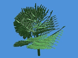
   L-systems, or Lindenmayer systems, were not invented to create fractals but to model cellular growth and interactions. A L-system is a formal grammar to transform, by iteration, a starting string of characters into another string. The transformation is based on rules that specify how characters or sub strings are substituted by others. By recursively applying the rules of the L-system to an initial string, a string with fractal structure can be created.
   Basically, each character can be a symbol having any conventional meaning, depending on what you intend to model. Very soon, L-systems have been applied to draw complex figures, each character being interpreted as a graphic command. The conventions used can be freely chosen in each program implementing L-system.
   The following example is quoted from the Fractint manual (by courtesy of Tim Wegner) and, therefore, use the particular syntax of this program. It draws the well known Dragon curve which illustrates the first page of each chapter of the book “Jurassic Park” by Michael Crichton:

Dragon   {       ; Name of lsystem, { indicates start
 Angle 8        ; Specify the angle increment to 45
                  degrees (360/8)
 Axiom FX       ; Starting character string
 F=             ; First rule:  Delete 'F'
 y=+FX--FY+     ; Change 'y' into  "+fx--fy+"
 x=-FX++FY-     ; Similar transformation on 'x'
 }              ; final } indicates end

   The standard drawing commands are:

F Draw forward
    G Move forward (without drawing)
    + Increase angle
    - Decrease angle
    | Try to turn 180 degrees. (If angle is odd, the turn
      will be the largest possible turn less
      than 180 degrees.)

dragon.gif (2215 octets)

Dragon curve after 10 iterations

Sierpinski { 
  axiom F+F+F
  f=F[+F]F
  angle 3
 }

Sierpinski triangle after 4 iterations ==>


   Prusinkiewicz is the initiator of the use of L-systems to model the logic of the plant structure (branching...). Many plants exhibit fractal patterns. L-systems are very useful for generating realistic plant structures, but can also be used to create strange and spectacular objects. The best results are obtained when the output of the program is processed by a ray-tracing program.

   Some references are:

  • P. Prusinkiewicz and J. Hanan, Lindenmayer Systems, Fractals, and Plants, Springer-Verlag, New York, 1989.
  • P. Prusinkiewicz and A. Lindenmayer, The Algorithmic Beauty of Plants, Springer-Verlag, NY, 1990. ISBN 0-387-97297-8. A very good book on L-systems, which can be used to model plants in a very realistic fashion. The book contains many pictures.
  • Tutorial about L-systems - David G. Green
    http://life.csu.edu.au/complex/tutorials/tutorial2.html


 3k

What are fractal terrains? 


   Drawing landscapes with computers was one of the first artistic uses envisaged for fractals. Mandelbrot himself has made some studies, and some other authors have written programs with spectacular results. Fractal landscapes have been used, for example, in Star Trek II. One of the best known creators of fractal landscapes is Ken Musgrave, who worked first with Mandelbrot.
   This topic is generally called “fractal terrains”. The use of fractals is obvious in this field because, if you travel or zoom in such a landscape, it will show you even more details owing to its fractal structure.
   The simplest algorithm, which has several variants, is named “midpoint displacement”. To understand this algorithm, it is better to start by drawing something resembling a ridge line in the horizon. The following pseudo-code and images are excerpts of the page by Paul Martz (by courtesy of the author; see reference below):

One-dimensional midpoint displacement is a great algorithm for drawing a ridgeline, as mountains might appear on a distant horizon. Here’s how it works:

Start with a single horizontal line segment.
Repeat for a sufficiently large number of times {
  Repeat over each line segment in the scene {
    Find the midpoint of the line segment.
    Displace the midpoint in Y by a random amount.
    Reduce the range for random numbers.
  }
}

How much do you reduce the random number range? That depends on how rough you want your fractal. The more you reduce it each pass through the loop, the smoother the resulting ridgeline will be. If you don’t reduce the range very much, the resulting ridgeline will be very jagged. It turns out you can tie roughness to a constant; I’ll explain how to do this later on.


First iteration

Third iteration

Final image
from http://www.gameprogrammer.com/fractal.html


   To have a 3D terrain, a plane is divided into several areas (squares for examples) by means of a mesh. A random vertical displacement (in a given range of values) is applied to the middle point of each area. Then, each area is subdivided in the same way (recursively)  and a random displacement is applied to the middle point of each resulting area, but the maximum range of this displacement is the initial range divided by some coefficient. The process is repeated a great number of times. Depending the grid used and the value of the coefficient, the generated surfaces give rather realistic and various images of terrains (of course the grid must not be drawn in the final image and the generated surface must be colored and post-processed by a ray-tracing algorithm).
   More sophisticated mathematics lead to more realistic landscapes. The following text consists of excerpts of a Ken Musgrave’s web page (by courtesy of the author; see reference below):

All successful synthetic terrain models for computer graphics are fractal: That is, they feature complexity resulting from the repetition of form over a variety of scales. The complexity resulting from this repetition of form over many scales leads to the odd idea of fractal dimension: a spatial dimension which is intermediate between the familiar integer-valued (i.e., 1, 2, and 3) dimensions we’re used to dealing with. Most fractal terrains are based on a fractal function called fractional Brownian motion or fBm for short. FBm is simply a sum of randomly phase-shifted sine waves, the amplitude of which varies with frequency as 1/fb for 1<=b<=3. FBm has a jagged trace which resembles the skyline of a mountain range. Mandelbrot observed this and reasoned that extending the function to two (-point-something, if you insist) dimensions would result in a surface resembling mountainous terrain. He did so and presto! fractal mountains were born.
...FBm is, by design, statistically homogeneous and isotropic. That is, while it is not exactly the same in any two places, it has the same “feel” everywhere. Real terrains are more complex than that.
...When I started working with him in 1987 Mandelbrot was interested in ameliorating some of the documented artifacts inherent in efficient fBm-approximation algorithms. Following his lead I developed some conjectures of my own concerning the morphology of terrain which lead to models which incorporate heterogeneity, e.g., valleys which are smoother than peaks. I had not yet heard of the term at the time, but these models were multifractals: heterogeneous fractals the heterogeneity of which is the same over a variety of scales.

   Explanations with illustrations can be found at:


 3l. 

What is fractal music? 


   In the strictest sense, Fractal Music is the term for music derived from fractal algorithms. Instead of iterating an equation and applying the results to color a pixel (as with fractal graphics), they are applied to audio parameters. Most common is to apply the results to MIDI parameters, though application to wav is not unheard of, and the proposed MP-4SA format may spawn many new applications. As with fractal imagining software, the actual mapping of equations onto musical parameters, subsequent filtering and other transforms are at the discretion of the software author. The scope of what can be created musically is as infinite as the realm of fractal graphics.

What types of fractal music are there?
   
The term has come to take on broad meaning, much like the term “coke” is applied to “softdrink”. Proponents of this music use the term quite liberally; indeed, even software authors incorporate a variety of algorithmic methods, including non-fractal methods of generation. Randomizing routines, Cellular Automata, RGB data from pictures, etc. have been used. One important note is that the term describes no specific genre of music, but rather a method of creating it.

Pure Fractal Music
   
This may not exist, since fractals are infinite and the music is finite. Also, in the least, there is a “fitting” to musical scale.

Workable Fractal Music
   
This is music generated using solely fractal maths, and necessary transforms to fit to a chosen scale. Examples would include MusiNum and Gingerbread.

Generative Music
   
This describes the majority of “Fractal Music” software. Fractal math is used, but a great many other algorithmic techniques are used, giving the software it’s own unique “flavor”.

Hybrid Fractal Music
   
The composer combines music generated by the above method(s) and adds music from other sources - conventional instruments, samples, other sounds. This approach seems most promising, as the composer has many tools at his disposal, and may mix and match at his discretion.

Non-Computer-Generated Fractal Music
   
Using a score from a Fractal Music piece generated by computer, this can be a starting point for further development using conventional instruments.

Fractal lullaby (created with Musinum by JPL)

Some links

Table of contents